
|
|
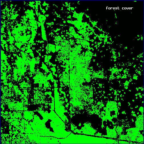
| Fig. A1. Forest cover in sample plot. | Fig. A2. Panther locations in sample plot. |
We begin with a small plot (15 km2) in our study area. The plot contains both forest cover (Fig. A1) and panther locations (Fig. A2). Estimating the fractal dimension (of either the forest or the subset of forest associated with panther locations) entails two steps.
 |
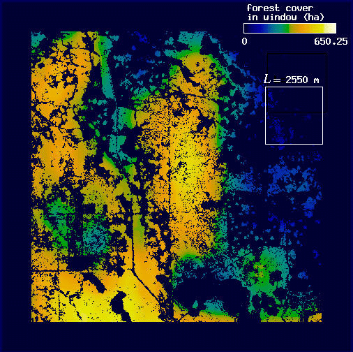 |
| Fig. A3. Map of forest cover for L = 450 m. Pixel values correspond to sum of forest area in window around the pixel (f). | Fig. A4. Map of forest cover for L = 2550 m. Pixel values are as in Fig. A3; the color scale is normalized to window width. |
Using these measures of forest cover at different window widths, we can estimate the fractal dimension of the forest cover in the plot. To do this, we first compute the mean value of all the forest pixels for each window width. For each window width L, we call the mean F(L). For L = 450 m, F(L) = 13.6 ha, whereas for L = 2550 m, F(L) = 346.9 ha. Because large windows only visit the center portion of the plot (note the increase in "border" from Fig. A3 to Fig. A4), we calculate F(L) using only those pixels visited by the largest windows. Values of F(L), collected in this way for many values of L, are then used to estimate the fractal dimension of the forest, D. A doubly logarithmic regression of F(L) on L generates a straight line, the slope of which provides an estimate of D (see Fig. 5).
For the conditional mapping analyses, we repeat the process just described, with two additional steps. We use the same values of L as before. First, we examine the distribution of panther locations (Fig. A2) and map all of the points associated with panther locations for a given value of L. To do so, we center a window on every pixel of the image and record whether a panther location occurs within the window or not. The proportion of the plot associated with panther locations changes drastically as we move from L = 450 m (Fig. A5) to L = 2550 m (Fig. A6). Thus, areas associated with panthers represent a more restricted subset of the plot at fine scales than at broad scales.
 |
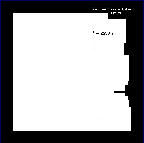 |
| Fig. A5. Map of all panther-associated sites for L = 450 m. | Fig. A6. Map of all panther-associated sites for L = 2550 m. |
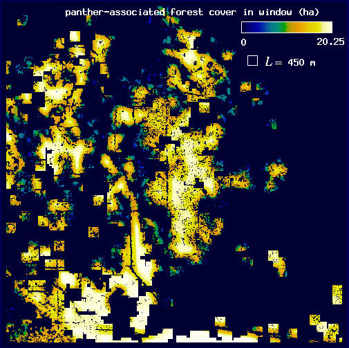
Next, we repeat this windowing procedure on the forest. Then, before calculating the mean amount of forest, we eliminate all of the forest pixels that are not associated with panthers, leaving behind the subset of forest associated with panthers for L = 450 m (Fig. A7) and for L = 2550 m (Fig. A8). Seen in this way, it becomes obvious that we are using the panthers as a filter on the forest image.
 |
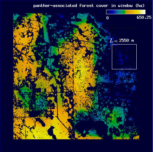 |
| Fig. A7. Map of forest cover associated with panther locations for L = 450 m. Pixel values are as in Fig. A3. | Fig. A8. Map of forest cover associated with panther locations for L = 2550 m. Pixel values are as in Fig. A4. |
Finally, we calculate the mean amount of forest associated with panthers, H(L), by taking the mean pixel value of all the forest pixels associated with panther locations for each value of L (for L = 450 m, H(L) = 14.8 ha, and for L = 2550 m, H(L) = 348.1 ha). We can then use these data to estimate the fractal dimension of forest areas associated with panther locations, E, using a doubly logarithmic regression of H(L) on L (see Fig. 8).