Nature vs. Nurture: the Making of the Montado Ecosystem

Paulo Miguel Pereira and Manuela Pires da Fonseca

• Abstract
• Introduction
• Methods
  • Study area and site selection
  • Data collection
  • Data analysis
• Results
  • Species richness and composition
  • Analysis of total variance: exploring who's who in shaping the montado ecosystem
  • Which variables are responsible for the patterns of plant and bird species distribution?
  • From the bottom up: how do individual species make up patterns of distribution?
• Discussion
  • Patterns of species richness and composition
  • What makes one montado different from another?
  • Which variables most affected plant and bird distribution?
  • How do individual species make up patterns of distribution?
• Speculation
• Conclusion
• Responses to this Article
• Acknowledgments
• Literature Cited

The southern Iberian Peninsula is dominated by a savannah-like ecosystem, the montado, which is a typically Mediterranean cultural adaptation to generally poor productive areas. Montados are exploited for three main uses: forestry, agriculture, and extensive grazing, in proportions that vary according to local conditions (more or less productive land) and historical circumstances. Because these ecosystems occur over a large geographic area (they occupy some 6 million ha), biodiversity would be expected to vary among montados. However, differences in management practices may also influence species distribution. In this paper, we investigate differences in plant and bird species diversity among 60 montados distributed all across southern Portugal. The environmental variables studied included geographical coordinates, climatological data, soil type, and altitude. We also investigated agro-economic variables that could describe human activities at each site: animal husbandry (breeds, stock density, grazing rotation, etc.), agriculture (fallow rotation frequency, use of fertilizers, etc.), and forestry (cork harvesting, thinning, etc.). Finally, land-use type and metrics were assessed from rectified aerial photographs. Species richness among these two groups was not correlated, sites with high or low numbers of plant species not necessarily having high or low numbers of bird species. However, both plant and bird communities exhibited a similar pattern of species composition and turnover. This pattern was ecologically based, rather than a result of biological similarities between groups: direct gradient analyses and variance partitioning revealed strong correlations between species distribution and spatial gradients, namely longitude and latitude. In trying to distinguish anthropogenic from biophysical processes, we found that both were equally important as drivers of montado biodiversity. Plants and birds exhibited a similar ecological pattern, although environmental conditions were slightly more important in the case of plants, and human activities were slightly more important in the case of birds.

KEY WORDS: biodiversity, birds, conservation, ecological concordance, human versus nature, montados, plants.

Published: May 13, 2003

The naturalness of extensive, traditional agro-forestry systems is often taken for granted (Pinto-Correia 1993, Herzog 1998a). Yet we are only starting to uncover patterns of biodiversity distribution, and hardly understand how land-use management affects wildlife as a whole (Santini and Angulo 2001). Recently, however, the suggestion that losses in biodiversity could be linked to intensification of agriculture or forestry has prompted an interest in understanding systems that have long been exploited by people (Pinto-Correia and Mascarenhas 1999). Such is the case of the montado, a traditional land use that covers about 6 million ha in the Iberian Peninsula. Given this wide geographical distribution, biodiversity necessarily varies among montados: for example, proximity to the coast versus a continental influence (e.g., Saetersdal and Birks 1993, Yeo and Blackstock 2002), and a latitudinal gradient (Gaston 1996) have been pointed out as robust patterns in species distribution. In this paper, we investigate patterns of plant and bird distribution across the 1175-ha area covered by montados in southern Portugal (Direcção-Geral das Florestas 2001).

A montado is an agro-forestry-pastoral ecosystem that consists of scattered tree cover (60–100 trees per ha) dominated by evergreen oaks (cork oak, Quercus suber, and holm oak, Q. rotundifolia), with pastures and agricultural fields (clover, wheat, barley, oats) as undercover, usually in a rotation scheme that includes fallows (Pinto-Correia 1993, Lourenço et al. 1998). It is a high diversity system (De Miguel 1999, Carrión et al. 2000), and the varying tree density suggests that these human-made agro-ecosystems have adjusted to local climate (Joffre et al. 1999). Shrubs sprout frequently (e.g., Cistus, Erica, Lavandula, and Ulex ssp.), and are either cleared out or artificially kept at low densities (Lourenço et al. 1998, Pinto-Correia and Mascarenhas 1999).

Recently, several authors have stressed the need to analyze and quantify the relationships between anthropogenic and non-anthropogenic factors in shaping ecological communities (Allen and O’Conner 2000, Yeo and Blackstock 2002), and Mediterranean ecosystems are especially suited to that purpose (Lavorel et al. 1998). Montados are listed in Appendix I of the European Community Habitats Directive (92/43/CEE). The fact that these ecosystems have been managed by humans for a long time (Joffre et al. 1999)—Iberian Romans reputedly bred pigs under evergreen oaks—makes them ideal cases to investigate the complex nature vs. nurture question.

In the Mediterranean region, human-induced changes are believed to account for an important part of the variation in the components and dynamics of current biodiversity (Lavorel et al. 1998, Blondel and Aronson 1999). Montados may be exploited for cereal cultivation, cork, charcoal, game, honey, meat, and dairy products, the latter usually being obtained from animals that are bred extensively. Some of these goals, however, may exclude each other. Shrubs may be used by game as shelter and by cattle as fodder, but they compete with the trees for water and nutrients; they also hamper the use of harvesters and balers. Pastures are generally poor, beginning to die out in May or June and, by the end of summer, acorns account for most of the diet of free-ranging animals. Cork oak acorns are economically less important than those of the holm oak (their tannin content is higher and they are less palatable), but the trees may also be exploited for cork. The choice of the main production goal, thus, is central to management (Coelho 1996). Land management, in turn, has been identified as a main driver of wild species distribution (Onipchenko and Semenova 1995, Leiva et al. 1997). Does nature still shape the biodiversity of the montados?

Previous studies have found a relative richness in montado bird diversity compared with other ecosystems. Yet no attempt has been made to systematically quantify and understand the drivers underlying this biological diversity. Nor have the ecological determinants of grasslands distribution, an ubiquitous presence in Mediterranean ecosystems, been thoroughly investigated (Azcárate et al. 2002). At a regional level, biogeographic and environmental factors have been described as the main determinants of plant diversity, but anthropogenic influence has also been identified at this scale (see Rey Benayas and Scheiner (2002) for the Iberian Peninsula and Yeo and Blackstock (2002) for Great Britain).

In this paper, we try to separate the anthropogenic factors from the natural factors that structure plant and bird diversity in montados. By collecting biological data through two independent sampling strategies, it was possible to validate the ecological models obtained. Biological concordance results from ecological coincidence between plant and birds; humans and nature shape the montado to an equal degree. An attempt was made to obtain a larger picture of montado ecology that will provide a basis for conservation planning and land management in the Alentejo region of southern Portugal.

Study area and site selection

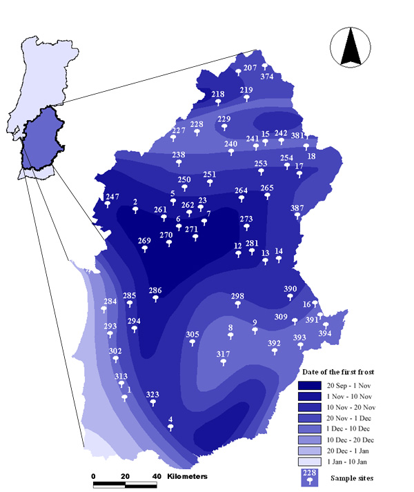
The study area encompasses the Alentejo region in southern Portugal (Fig. 1). This area was chosen because it encompasses over 1 million hectares of montados, a large enough area to enable the investigation of contrasting ecological forces. Data were collected during 1998 and 1999 at 60 sampling sites distributed all across the study area (Fig. 1). Sites were selected using the European Community Forestry Monitoring 16 x 16 km grid, with the resolution increased to 8 x 8 km with the help of a geographic information system (GIS). Within this systematic grid, and with the help of an agro-forestry map, we chose 100 intersections at random as potential sites, verified them all in the field, and selected 30 that were cork oak-dominated montados and 30 others that were holm oak-dominated montados. This stratification ensured equal representation of both oak species. Montados thrive under the typical Mediterranean climate of long, hot, dry summers (daily maximum temperature often reaches 40ºC) and mild, humid winters (average rainfall of 500–650 mm) (Instituto Nacional de Meteorologia e Geofísica 1991), varying from the milder conditions along the ocean shore in the west, to the more extreme continental east (Rey Benayas and Scheiner 2002).

Fig. 1. Sampling site locations in the Alentejo region, southern Portugal, superimposed on an Eco variable, namely date of first frost (data obtained from the Portuguese Meteorological Service).

Data collection

One way to analyze the impact of human activities on an ecosystem is to identify and quantify the agro-economic activities (cork harvesting, herding, and cereal cultivation, for example) that characterize each site. Another way is to look for patchiness resulting from different land uses and, therefore, we also used landscape metrics as explanatory variables. Thus, we had two separate sets of human-induced variables which, together with a set of environmental variables, were used as explanatory variables to identify the driving forces underlying montado species composition and diversity. A systematic field survey of plant and bird species was performed in 1998 and 1999 at 60 sampling sites distributed across the study area (Fig. 1).

Four sets of variables were collected: the Bio, Eco, Land, and Ae sets.

1. The Bio set. Two biological groups were surveyed: plants (species composition and percentage of cover intensively surveyed within a 100-m circle centered on the sampling site centroid, plus identification of all species on a transect within a 1-km radius) and birds (three point counts per 1-km radius, twice in spring and once in winter in 2 consecutive years). In the case of plants, the dependent variable represents plant cover (measured on a 1–6 logarithmic scale). For birds, it represents frequency of observations, ranging from one (species seen only once) to 18 (species seen in all three point counts in each of the three seasonal counts, in both years).

2. The Eco set (Table 1, 22 variables). Environmental variables included climatological data (Comissão Nacional do Ambiente 1983, Instituto Nacional de Meteorologia e Geofísica 1991) (e.g., temperature—maximum and average; frost—number of days between first and last frost; date of first frost—see Fig. 1), soil type (pH was obtained from soil samples in the lab), altitude (obtained using military maps), and geographic coordinates (assessed locally with a global positioning system (GPS)). Spatial variables were included in the analyses because they may act as synthetic surrogates for environmental parameters that are difficult to measure directly (Borcard et al. 1992, Borcard et Legendre 1994, Yeo and Blackstock 2002).

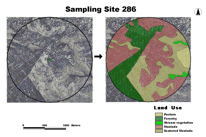
3. The Land set (Table 1, 24 variables). The variables were land use and landscape metrics (Fig. 2). Land-use types were identified on rectified aerial photographs (1:33 000) and validated in the field (Fig. 2); landscape metrics were extracted within a 1-km radius circle, from rectified aerial photographs (1:33 000), using the Patch Analyst extension of ArcView (Elkie et al. 1999).

4. The Ae set (Table 1, 33 variables). Agro-economic variables described local economic activities: animal husbandry (breeds, stock density, grazing intensity, etc.), agriculture (fallow rotation time, use of pesticides and fertilizers, etc.), and forestry (cork harvesting, thinning, etc.). These variables were obtained through questionnaires sent to the owners and land agents of each of the sites, which were filled in with the help of a research team member. The Ae variables list was rounded out with information collected directly in the field. All this information was stored in a GIS.

Fig. 2. Example of Land variables generation: land-use types within a 1-km radius circle (Sample Site 286), extracted from aerial photographs. The arrow describes the process of photo interpretation.

Data analysis

1. Alpha diversity patterns were accessed calculating plant and bird species richness at each site; the correlation between plant and bird species richness (number of species per site) was tested using Spearman’s correlation test (Sokal and Rohlf 1995).

2. Concordance of plant and bird species composition patterns was investigated by running a Mantel test in the PRIMER statistical package (Clarke and Gorley 2001). The Mantel test used Pearson's correlation to relate the two distance matrices (plants and birds) obtained with Bray–Curtis distances (the calculated distances measured the distance between sites based on plant and bird data); a significance level was obtained after 9999 permutations using the Monte Carlo randomization method.

3. Multivariate analysis was used because matrix algebra perfectly fit the nature of large biological and ecological data sets: sample plots are represented in columns, species or explanatory variables in rows (Legendre and Legendre 1998). A preliminary detrended correspondence analysis (DCA) (Hill 1979) (run with all species data and by biological group) revealed comparatively short lengths of gradient, which indicates that non-unimodal responses to environmental variables would be expected for most species (ter Braak and Šmilauer 1998). Thus, assuming that most species would exhibit a linear response to the explanatory variables, we proceeded with a constrained ordination using canonical redundancy analysis (RDA) (Jongman et al. 1995, ter Braak and Šmilauer 1998).

4. The total number of explanatory variables (n = 79) was reduced by selecting, within each data set, the 14 best explanatory variables; this number was reduced to eight variables for each set, by eliminating all variables that were strongly autocorrelated in each data set (see Appendix 1). One variable was eliminated (us-la: stream vegetation land-use) because, although vegetation sampling included this habitat, bird sampling excluded it. The equal number of variables in each group ensured that the three sets of explanatory variables could be compared, and that their variance would not be related to the number of variables within each set (following Paszkowski and Tonn 2000); subsequent analyses used only 24 variables.

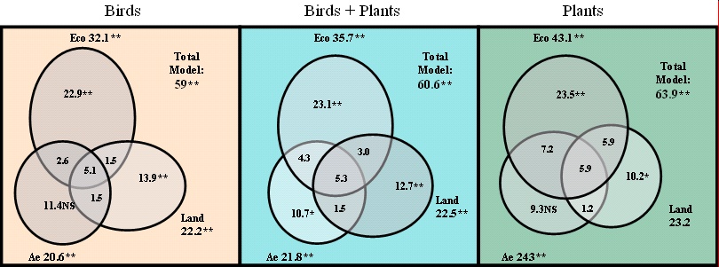
5. In order to distinguish the importance of each of the three sets of explanatory variables in structuring the montado ecosystem, a Partial RDA (Borcard et al. 1992) was run; this type of analysis was thought appropriate because it allows variance partitioning between groups of variables (two groups: Borcard and Legendre 1994, Paszkowski and Tonn 2000, di Giulio et al. 2001, Heino 2001; three groups: Magnan et al. 1994, Yeo and Blackstock 2002), therefore, making it possible to investigate the relative importance of each of the three independent data sets (Eco, Ae, and Land) in explaining biological diversity. The methodology used to assemble the variance partitioning is explained in Fig. 3; the significance of each model was tested using Monte Carlo permutation tests for both the first axis and the full model (Jongman et al. 1995). The variance partitioning was first carried out with all biological data together; we then ran independent models with data on either plants or birds only, in order to identify the biological group responsible for the observed pattern.

6. In order to explore the behavior of the most significant species in RDA in relation to the most significant environmental variables in that same RDA (latitude and longitude), multinomial logit models (McCullagh and Nelder 1989) were adjusted for each species using the canodraw module of CANOCO; we adopted a generalized linear model (GLM) approach instead of using simple linear regressions, because the former allows for the identification of the type of response (monotonic, unimodal, bimodal, etc.) of the species along the studied environmental gradient. Significant species were those with p < 0.001. Analyses iii, iv, v, and vi were performed using CANOCO for Windows, version 4.02 software (ter Braak and Šmilauer 1998).

Fig. 3. Methodology to assemble variance after partitioning (partial RDA): schematic representation and calculation procedures. “/” means “covarying out;” e.g., “Eco/Ae + Land” means “Eco set covarying out Ae and Land sets.” Variables are in orange and covariables in green.

The Bio set comprises 14 000 identified plants (596 species) and 17 000 sightings of birds (128 species). The explanatory variables collected amounted to 79 (Table 1); this number was reduced to 24 (Table 3) and subsequent analyses used these 24 explanatory variables only. Other authors have successfully reduced a larger set of variables to seven, in order to standardize groups of factors in partial RDA (Paszkowski and Tonn 2000). To the best of our knowledge, the present study provides the first clear compositional and ecological concordance of plants and birds in an ecosystem; Woinarsky et al. (2001) found a relationship between bird species composition and plant grouping, but each distribution was explained by a different ecological driver.

Species richness and composition

The species richness of plants and birds was not correlated: sites with high plant diversity did not have high bird diversity, and vice versa. The results of the Spearman correlation test (R = 0.063; p = 0.96) do indicate a random relation between the two groups. However, the Mantel test result was highly significant (Rho = 0.202; p = 0.0005), uncovering a clear turnover similarity in plant and bird species distribution: Bray–Curtis distances between the 60 sites showed practically the same biogeographic pattern for the two groups.

Analysis of total variance: exploring who’s who in shaping the montado ecosystem

Variance partitioning suggests that humans (Ae and Land, the two sets of anthropogenic variables together covarying out Eco) account for as much of the variance in global biodiversity (plants + birds) as nature (the Eco set covarying out Ae and Land) (Fig. 4) (For calculations, see Fig. 3: humans=2+3+C and nature=1; thus, in Fig. 4, humans=10.7+12.7 +1.5=24.9% and nature=23.1%.) The full model explained 60.6% of the variance: both the model and the first axis were significant (please refer to Fig. 4 and Table 2). Each of the three sets of explanatory variables was significant on its own. The Eco variables explained 35.7% of the total variance, the Ae variables 21.8%, and the Land variables 22.5%. In the Eco set, this percentage fell to 23.1% when covarying out the Ae and the Land variables (this figure is still highly significant, and it corresponds to eight variables being covaried out by 16). In the Land set, the percentage fell to 12.7% when the Eco and Ae variables were covaried out but, again, was still very significant (p < 0.0001). In the Ae set covaried out by the Eco and Land variables, variance fell to 10.7% and this value was almost nonsignificant (p = 0.0403). In fact, most relationships were actually found to be highly significant: after 9999 Monte Carlo permutations, all relations were found to be significant: eight with p < 0.0001, one with p < 0.01 (in the Land set), and three with p < 0.05 (in the Ae set) (Table 2).

The model improved when run with data on plants only (63.9% of the variance explained; Fig. 4). In this case, the environmental (Eco: 23.5%) surpassed the anthropogenic variables (Land+Ae=20.7%) in explaining species distribution. The Ae set of variables, significant on its own, was nonsignificant when covaried out by the Eco and the Eco+Land variables; most of the variance apparently explained by management differences was in fact induced by ecological and structural (landscape) constraints.

When restricted to bird data, the model explained 59% of the variance (Fig. 4). With birds, anthropogenic variables exceeded environmental ones (25.3 and 22.9%, respectively) in explaining species distribution. However, the set of agro-economic variables, significant on its own, was nonsignificant when the other two sets of variables were covaried out (Fig. 4). As with plants, the physical structure of the ecosystem and ecological variables seemed to be the main driver of bird distribution.

Fig. 4. Results of the partial RDA with three sets of explanatory variables for two biological groups, both individually and combined (see Fig. 3 for scheme; Table 2 explains the significance). NS: p > 0.05; *: p < 0.05; **: p < 0.001.

From the variance partition diagram (Fig. 4), it is evident that the three set of variables were fairly independent, with the ratio between interaction variance (A+B+C+D in Fig. 3) and pure variance (1+2+3 in Fig. 3) being 1:3.

Which variables are responsible for the patterns of plant and bird species distribution?

In the global model for plants and birds, all 24 variables were significant to at least one model (Table 3).

Among these, the ten most explanatory variables were significant for plants and birds: in both cases, longitude (COO_X), latitude (COO_Y), temperature (ab-temp), precipitation (ab-prec), humidity (ab-hum), minimum altitude (ALT_MIN), podzols (ab-pdz), cork extraction (Ae-de), forestry (us-pl) and over-scattered montado (us-mdd) were significant, explaining a similar amount of variance (see Table 3). These ten variables alone explained 46.1% (plants) and 35.4% (birds) of the total biological variance (Table 3). However, relevant differences were found between the two biological groups. In the Eco set, altitude (ALT_MIN) and podzols (ab-spz) explained much more variance in plants (8.9 and 11% more variance, respectively), but climatological data better predicted bird species variation (see Table 3). In the Ae set, cows (ae-bov), compensatory measures (ae-cp), fertilizer type (ae-tad), abandoned farms (ae-mdes), and goats (ae-cap) were significant for plants but not for birds, and fire (ae-fl) and cereal (ae-CS) exhibited the opposite pattern. Finally, in the Land set, land use was significant for birds but not for plants (except for over-scattered montado and forestry), and landscape metrics were significant only for plants (see Table 3).

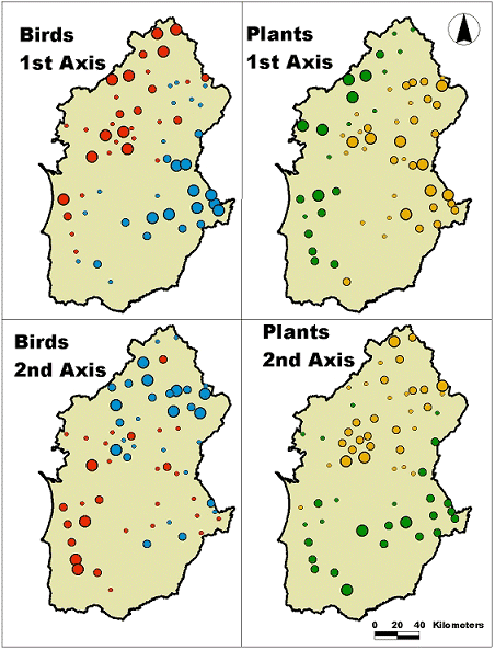
Our results suggest that montado biodiversity is largely controlled by spatially structured environmental gradients. As the two most important explanatory variables turned out to be geographic coordinates, it was possible to plot the sample scores on the 1^st and 2^nd axis of each group’s RDA. It then became clear that plant and bird species showed similar turnovers following a west–east gradient, defined by the 1^st axis, and a south–north gradient, defined by the 2^nd axis (Fig. 5). Given this coherence, we chose to investigate how the main ecological gradients (N–S, E–W) conditioned plant and bird distribution by producing a GLM for individual species.

Fig. 5. Projections of sampled sites on the 1st (18.1% of explained variance for birds and 25.8% for plants) and 2nd axes (8.8% of explained variance for birds and 8.3% for plants) of the RDA for both birds and plants. Scores are indicated by color: blue and green are positive, red and yellow are negative; dot size is proportional to sample scores.

From the bottom up: how do individual species make up patterns of distribution?

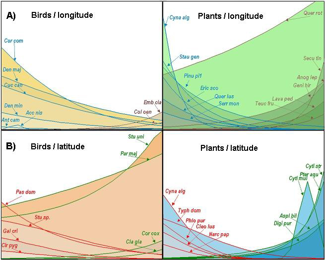
In the case of plants, when latitude was used as the explanatory variable, the GLM confirmed a clear turnover of species: some plants were restricted to or predominated in the south (41 species, e.g., Cynara algarbiensis, Typha domingensis, Phlomis purpurea, Cleonia lusitanica, Narcisus papiraceus in Fig. 6), some in the north (13, e.g., Cytisus striatus, Pteridium aquilinum, Asplenium billoti, and Digitalis purpurea), some had a unimodal behavior (seven, e.g., Cytisus multiflorus, but completely unbalanced to the north), and one had a bimodal behavior (see Appendix 2 for the complete species list).The turnover that followed an increase in longitude was even clearer, with species predominating in the west (75 species, e.g., Cynara algarbiensis, Stauracantus genistoides, Pinus pinea, Erica scoparia, Quercus lusitanica, and Serratula monardii in Fig. 6), although some were restricted to or predominated in the east (31 species, e.g., Quercus rotundifolia, Securinega tinctoria, Anograma leptophylla, Genista hirsuta, Lavandula pedunculata, and Teucrium fruticans in Fig. 6); only one species showed a unimodal behavior.

Fig. 6. A) GLM using longitude as the explanatory variable (represented in km on the X axis); the Y axis represents plant cover (1–6) and bird frequency (1–18). The blue lines represent species that were more abundant in the west; brown lines represent species that showed a preference for the interior. B) GLM using latitude as the explanatory variable (represented in km on the X axis). The red lines represent species that were more abundant in the south; green lines represent species that showed a preference for the north. Species labels are abbreviated. See main text for a complete description.

Bird distribution was also latitude–longitude related, but the number of significant species was much lower. From west to east, communities dominated by forest species (six species: Anthus campestris, Corvus corone, Cuculus canorus, Dendrocopos major, and Dendrocopos minor; Accipiter nisus was unimodal, but predominated in the west) gave way to communities of open-habitat birds (two species: Columba oenas and Emberiza cia). Within these communities, some species were consistently found in the north (four species: Clamator glandarius, Corvus corax, Parus major, and Sturnus unicolor), whereas others were characteristic of the south (four species: Galerida cristata, Circus pygargus, Passer domesticus, and Sturnus ssp.) (Fig. 6).

Our aim here was to investigate the diversity of montado plant and bird species and its dependence on ecological gradients. Despite differences in species richness (Spearman correlation test was nonsignificant), the two biological groups showed changes in community composition that were significantly related (Mantel test highly significant). Moreover, the pattern of species turnover observed for each biological group was explained by a similar set of ecological factors (partial RDA gave similar models and the ten best explanatory variables were significant for both groups). A similarity in patterns of distribution has been found previously and explained on the grounds of specific relationships between groups (mutualism: see Eastwood and Fraser (1999); predator–prey: see Cotton 1998). A few authors, however, suggest that common patterns may simply result from the fact that different groups of organisms may react in the same way to the environment (Catterall et al. 2001). We found that plants and birds distribute themselves in a similar fashion, and we further tried to understand whether their geographic distribution patterns were ecologically or human driven.

Patterns of species richness and composition

The diversity patterns of the two biological groups did not match: species richness showed an independent behavior for plant and bird species, challenging previous work that used only one biological group as a surrogate for diversity (see Duelli and Obrist (1998); but see also Jonsson and Jonsell (1999) and di Giulio et al. (2001)). Although high numbers of species do not necessarily mean high conservation value (Duelli and Obrist 1998), the quest for relationships between biological distributions usually aims at finding indicator species for conservation purposes (Jonsson and Jonsell 1999). Our results clearly showed that, in the case of montados, a conservation strategy aimed protecting plants would not necessarily protect bird species, and vice versa. Several authors have acknowledged the fact that care has to be taken when applying simple estimates for decisions on conservation measures (Jonsson and Jonsell 1999).

The Mantel test showed that the ecological pattern observed was a result of a similar turnover in species composition across the 60 sampling sites; this test was run with biological data only, revealing that the distances among sites based on either plants or birds were similar. The fact that this test was independent of the partial RDA adds reliability to the observed pattern. A similar concordance in ecological patterns has been found between apparently unrelated biological groups, such as birds and fishes (Paszkowski and Tonn 2000); birds, plants, and invertebrates (Catterall et al. 2001); macrophytes, dragonflies, stoneflies, diving beetles, and fishes (Heino 2001); vascular plants, bryophytes, and lichen (Pharo et al. 1999). That plants and birds responded equally to anthropogenic and environmental variables may reflect the long coexistence of humans and nature in Mediterranean regions (Blondel and Aronson 1999).

What makes one montado different from another?

The results of variance decomposition using both plant and bird data revealed that anthropogenic (the Land and Ae sets) and environmental (the Eco set) factors were responsible for the observed patterns of biological distribution (see McIntyre and Martin (2001), for a similar result in Australia, in this case with richness measures). The driving force of anthropogenic actions upon species distribution has recently been reported for birds (Freemark and Kirk 2001, Allen and O’Conner 2000), plants (Yeo and Blackstock, 2002), and insects (di Giulio et al. 2001).

In this study, strong emphasis was placed on the use of variance partitioning to elucidate the relative importance of each of three groups of explanatory variables. Our partitioning of variance had a ratio interaction: pure variance of 1:3 (Yeo and Blackstock (2002) obtained a ratio of 7:5), which accounted for the independent character of the three groups of variables, the independent variance of each group being much higher than the interaction between all groups, indicating that they are clearly separable in their effects (Borcard et al. 1992). Also, by analyzing the three sets of variables together and on their own, it became clear how misleading the choice of explanatory variables might be. For instance, although we found that the agro-economic variables explained 20.6% of bird diversity (p < 0.0001) and 24.3% of plant diversity (p < 0.0001), the variance partitioning allowed us to understand that part of that variance was in fact correlated with other groups of variables (Eco and Land), and the resulting partial model (Ae covarying out Eco and Land) became nonsignificant. Autocorrelation between explanatory variables is probably unavoidable in ecological studies, although it is of utmost importance to uncover these masking relationships. Thus, analyses that clearly separate and quantify slices of explanatory variance seem to provide an approach closer to real ecological processes than more simplistic approaches that use a single biological group, or a single set of explanatory variables.

When the two biological groups were analyzed separately, birds seemed to be more affected by anthropogenic variables (see also Freemark and Kirk (2001), Mitchell et al. (2001), Allen and O’Conner (2000)), and plant distribution was more affected by the ecological set (see Saetersdal and Birks (1993), Forbes et al. (2001), Yeo and Blackstock (2002)). The response of birds to landscape structure has been reported before: some authors have noted bird species restricted to certain land uses (e.g., farmland birds (Chamberlain and Fuller 2001, McIntyre and Martin 2001)). The density of tree cover, one of the variables that best explained bird distribution (in our study, it was represented by the variables us-mo, us-md and us-mdd), has been shown elsewhere to determine the distribution of parrot species (Marsden and Fielding 1999).

As for the response of the biological data to the explanatory variables in partial RDA, Fig. 4 clearly shows that the pattern drawn by each biological group matched the one obtained with all data together. Because the sampling procedures adopted to survey each biological group were independent, either group may be used to validate the global model produced: this cross-validation is essential in multivariate analyses in order to ensure that the data are robust, and that the pattern identified could not have been obtained by chance alone (Legendre and Legendre 1998). Moreover, the two independent data sets were explained by a similar set of variables (in the respective independent models, the ten best variables were significant for both groups); such a result proved that those variables were responsible for a true ecological pattern, and were not merely the result of a type II error (Sokal and Rohlf 1995) during the selection of environmental variables. This coincidence of distributions may not be a consequence of similar processes affecting different groups, but rather of covariation within a wide range of ecological and anthropogenic factors (Catterall et al. 2001).

Which variables most affected plant and bird distribution?

The results obtained with the full model (24 explanatory variables), showed latitude and longitude as the main drivers of plant and bird species distribution (Table 3). Geographical gradients in species diversity are almost universal across taxa (Lennon et al. 2000) even at small scales (Bogya et al. 1999). For example, latitude has been shown to explain an increase in species richness at continental scales (Gaston 1996), and both latitude and longitude explain species composition turnover at regional scales (O’Hara and Poore 2000, Heino 2001, Yeo and Blackstock 2002). Our understanding is that, in our analyses, these variables stand out as unintentional surrogates of other environmental variables (e.g., proximity to the ocean, see Satetersdal and Birks (1993), O’Hara and Poore (2000), Yeo and Blackstock (2002)). Indeed, geographic coordinates are strongly correlated with environmental variables (see Appendix 1).

One other variable followed in importance: cork extraction (ae-de), a variable meant to quantify cork exploitation. Cork extraction is carried out (by hand) on scattered trees only every 9 years, so it can hardly disturb plants or birds. The shrub layer is left at relatively higher density in cork oak montados than in holm oak montados (Lourenço et al. (1998) give percentages that vary from 6 to 30% cover). The fact that shrubs explain most of the variance in plant distribution in montados, perhaps helps explain differences ascribed to the variable cork extraction. For birds, differences in area of shrub cover may represent significant differences in landscape structure and, thus, the 7.9% variance found. Cork oak predominates in coastal areas (southwest Portugal) and, in fact, ae-de was autocorrelated with longitude (see Appendix 1). Our results agree with a general understanding that the restricted cork oak distribution area of today is probably ecologically driven (ae-de was strongly correlated with many environmental variables: COO_X, ab-pH, ab-evap, ab-sol, ab-prec and ab-spz; see Appendix 1). The loss of significance in the Ae model when covarying out Land and Eco variables is probably related to this correlation. And, most probably, it should be the cork oak forest together with the ecological gradient that is mainly responsible for the variance explained in both groups.

Edaphic idiosyncrasies could explain particular plant assemblages, as podzols (ab-spz) imply siliceous/acid substrates (Natividade 1950, Ojeda et al. 1995); this explains the huge differences found in podzol variance (14.7% for plants and 3% for birds), because podzols mostly affect plant distribution, being the habitat of heathland species (Ojeda et al. 2000). Variable ab-spz can also act as a surrogate for the influence of the Tagus basin, as all podzol sites are located there.

The elevation gradient was also found to be significant, although it explained considerably more of the variance in plant than in bird distribution (12.6 vs. 3.7%). Kessler et al. (2001) suggest that peaks of plant richness in altitude are probably due to solar radiation and ecosystem productivity. Although the range of altitude we studied (25–450 m) is considerably less than that studied by Kessler et al. (2500–4000 m), our results also confirmed that altitude primarily affects vegetation cover (see also Lobo et al. (2001) for the Iberian Peninsula). Catterall et al. (2001) identified altitude as a driver of biologic turnover at only 35 m, finding that altitude was a surrogate for distance to the drainage lines. In the Mediterranean region, where water availability is an important limiting factor, altitude may lead to very distinct habitats on opposite hillsides (Heywood 1960, Sternberg and Shoshany 2001): slopes receiving higher solar radiation usually get less rainfall (Kadmon and Danin 1999), which translates into higher daily maximum temperatures and higher evapotranspiration rates (Sternberg and Shoshany 2001). Frost distribution and temperature were indeed factors that successfully explained plant and bird distribution (Table 3) (see, e.g., Bannister and Polwart (2001)). Apart for the cork extraction variable explained above, five other anthropogenic variables seemed to affect plant distribution (Table 3). (i) The presence of goats and cows, which are recognized to influence vegetation cover and composition (Lourenço et al. 1998, Ritchie and Olff 1999, Vesk and Westoby 2001). In the case of montados, goats may determine shrub and oak cover density, for they ultimately control natural regeneration and specimen size (Lourenço et al. 1998). (ii) Compensatory measures, which are directly related to the livestock pressure in montados (see Pinto-Correia and Mascarenhas (1999)). (iii) Fertilizer type directly affects plant species composition, with specialist and intolerant species being replaced by generalist and tolerant species in response to fertilization (see McIntyre and Martin (2002)). (iv) Abandoned farms, most probably resulting from this variable being negatively correlated with cows and fertilizer (see Appendix 1).

The only land use more related to plants was forestry. The main trees used in forestry are the maritime pine (Pinus pinaster) and the Eucalyptus (Eucalyptus globus). Pine forests are home to many plant species not found in montados. Eucalyptus forests, however, are usually barren of plants. In both cases, forestry affects plant turnover. Birds are also affected by forestry, for the same reasons given above and because there are bird species specific to pine forests. Almost all bird species avoid Eucalyptus forests.

The higher number of plant species in relation to bird species in GLM turnover can be interpreted in light of the different ecological requirements of the two biological groups. Unlike plants, bird population distributions are best considered from a landscape perspective (Askins 2000, Mitchell et al. 2001). Despite differences among the montados studied, in a broad sense they all fall in the same category of a savannah-like landscape, that is, they all represent one type of habitat. However, birds did respond to several anthropogenic variables (Table 3), particularly those concerned with density of tree cover (us-mo, us-md, us-mdd; important for birds that live on trees), and the type of ground cover (ae-CS, agriculture, us-pa, pasture; offering different diets, thus attracting different bird species). ae-fl (fire presence in replicates) affects both tree and ground cover when present, thus directly affecting bird species. Our results agree with previous work that found birds related to land use (Allen and O’Conner 2000, Mitchell et al. 2001) and to vegetation structure (Moreira 1999, Perkins et al. 2000), but the nonsignificant landscape metrics are surprising. The reason underlying this pattern resides in the nature of montado landscape metrics: apart from stream vegetation, there are no proper edges but rather gradual boundaries, thus not significantly affecting bird ecology. Landscape metrics mostly affected plant distribution, because the edges between patches can harbor many plant species and, essentially, because of the correlation to the stream vegetation (responsible for 10.2% of plant variance). This habitat forms long patches and strongly affects landscape metrics. Despite its exclusion from the final set of variables (because bird sampling did not include this habitat), we think that it provides interesting results for plants and, with proper sampling, it should provide the same good results for birds.

Differences among these variables are mainly due to management options, and these are not based on geographic grounds. In spite of this, we succeeded in finding a geographic pattern for bird distribution across the Alentejo. This pattern is evident in Fig. 6, where the cartographic representation of the two first axes in RDA for plants and birds shows a spatial continuity in the variance explained.

From this detailed analysis, it is evident that plants and birds throughout the montado landscape are best predicted by ecological variables, having more different responses with respect to anthropogenic variables (see Table 3).

How do individual species make up patterns of distribution?

There was a clear asymmetry in plant response to geographic coordinates, with many more species in the south and the west and a gradual impoverishment toward the north and the east (Table 4; Appendix 2). This asymmetry implies that richness measures in west vs. east montados and south vs. north montados are not comparable: west and south montados have many more species than east and north montados, and these might be a “natural” pattern. Birds concorded with plants with respect to longitude (more species in the west and fewer in the east), but showed the same number of species in the north–south gradient (Table 4; Appendix 2). When compared with plants, birds have fewer species responding to latitude–longitude gradients. In relative numbers (number of species responding to the gradient/total group species), only 6% of birds respond to latitude and longitude, but 9.1 and 17 .8% of plant species respond to latitude and longitude, respectively (Table 4).

This result apparently contradicts the RDA results (see Table 4). Although plant species responding significantly to latitude–longitude gradients were proportional to the explained variance in RDA, bird species, comparatively, had half the significant species in GLM analysis of what was expected after the explained variance in RDA (Table 4). A possible explanation for this result is that plant gradients along geographical coordinates better fit a non-linear response. This is reinforced by the length of the gradient expressed in DCA analysis (Table 4), with plants having a greater length than birds (plants with 2.005 s.d. and birds with 1.638 s.d.; Table 4). This reflects a better fit of birds to the linear model (thus RDA gave good results for birds) and plants approaching the unimodal model (better GLM models), yet considered preferentially a linear response (good RDA performance): the empirical limit to consider a better adjustment to the unimodal model is a gradient length greater than 3 s.d (Jongman et al. 1995).

The understanding that montados are not just a monotonous human-driven collections of grasses, shrubs, and oaks, but rather they include a number of ecologically meaningful and distinct species assemblages, is of utmost importance for nature conservation. Indeed, our results suggest that, by preserving a given montado, we can ensure the conservation of a given set of species. For instance, using the examples of the restricted range of species mentioned above (Fig. 6), by conserving the montados that occur within the distribution area of Genista hirsuta and Cynara algarbiensis, we can promote the persistence of these species. Identification of the main drivers of biodiversity distribution in the Alentejo allowed us to circumscribe biodiversity spatially, addressing a major problem in conservation biology (Santini and Angulo 2001): the fact that biological entities such as ecosystems lack discrete boundaries.

The question of nature vs. nurture is one of utmost importance in a region whose main environmental problems (degradation and desertification) have been ascribed to a long succession of civilizations, problems whose mitigation is now sought after by investing in land-use regulations (Pinto-Correia 2000). However, without understanding the dynamics of ecosystems, we can only guess which policy will achieve whichever goal we seek. Some authors claim that there is a clear benefit to be derived from extensive agricultural management as opposed to a more intensive one (see Herzog (1998b), Chamberlain and Fuller (2001) Freemark and Kirk (2001), di Giulio et al. (2001)). In the case of montados, although we did find that management clearly influenced species composition, the relationship between biodiversity and sustainability has yet to be established.

Land use is sustainable when, over generations, it supports the natural regulatory functions of ecosystems (biotic, abiotic) while allowing for profitable economic activities and providing an environment that enhances the physical and mental well-being of the people who live in it (Barret 1992). Montados do seem to fit the description (De Miguel 1999), but how do we measure deviations that become unsustainable? We have found that plants and birds at least distribute themselves in accordance with ecological gradients. Also, we have found differences in diversity among sites: montados with a high diversity of birds and low diversity of plants, vice-versa, and all conditions in between. We speculate, however, that it is possible to group montados into ecological types characterized by a number of indicator species (species indicator of a montado type, and not of high or low diversity). None of the studied montados looked degraded (although it was not our intent to study sustainability, therefore, we have no measurable definition of degradation), in which case these species would indicate types of sustainable management. A montado lacking the bioindicators of the type it should belong to, could be said to be at risk. For policies aimed at biodiversity conservation, looking at the specific assemblages that reflect the ecosystem as a whole would probably be preferable to quantifying species richness or diversity indices. From our data, it looks as though a montado may have a low biodiversity and still be the best possible option for a given area, in the sense that the absence of many species may be ecologically driven and not a result of mismanagement.

Our results showed that, despite long-term human intervention in montados (Joffre et al. 1999, Rey Benayas and Scheiner 2002), nature still plays a role in shaping this ecosystem. Reviewing the available palynological data for southern Iberia, Carrión et al. (2000) confirmed the presence of sclerophylous Quercus-dominated assemblages since the mid-Holocene. Interestingly enough, the floristic composition of those communities matches present-day Q. suber forests (Ojeda et al. 1995. Pérez-Latorre 1996, Lourenço et al. 1998, our own data). These thickets of shrub forest, which survive solely in land adjacent to montados (streamside tracts of land, stony uncultivated areas, quickset hedges), confirm that the monospecific cork–holm oak ecosystems are a result of human intervention (Joffre et al. 1999, Carrión et al. 2000). In the absence of human intervention, and given that the ecosystem still holds some resilience, the tree and shrub layers of montados will probably become more diverse. Indeed, of the total Iberian Peninsula fauna and flora, montados harbor circa 30% of the plant species, and 40% of the bird species (De Miguel 1999). These thickets may act as sources of natural material for the humanized montados: most plants belonging to this habitat were responsible for the observed turnover in species composition in the studied montados. Also, it seems worth investigating the importance of ecological corridors in spreading this continuous natural input. Low-diversity montados are common (as much as high-diversity montados) and part of the natural order and, above all, they contribute to the mosaic of different types of ecosystems that characterize the Alentejo: this patchiness of the landscape is crucial for many wide-ranging species.

Concordance between plants and birds was unequivocal from the agreement of the results of the Mantel test (only biological data), the partial RDA (with explanatory variables), and the ten best variables that were significant for both groups. This last result reciprocally validated the ecological models: out of the 79 initial variables, the fact that the ten best explanatory variables were significant for plants and birds could never be obtained by chance alone. Nevertheless, there were differences in the ecology of plants and birds: the former responded more to landscape metrics and grazing pressure by herbivores, while the latter responded more to land use.

Our results showed that humans and nature contribute in equal parts to the making of montados: the environment providing the raw ecological material, and humans decoding and exploiting it. Although this coevolution has been suggested before (Di Castri 1981, Blondel and Aronson 1999), to our knowledge this is the first quantitative attempt to distinguish between biophysical and anthropogenic processes in shaping this ecosystem.

Responses to this article are invited. If accepted for publication, your response will be hyperlinked to the article. To submit a comment, follow this link. To read comments already accepted, follow this link.

Data used in this paper were collected for the Project PAMAF 8151 “Methodological approach to identify and monitor biodiversity indicators for cork and holm oak montados at the management unit”; we thank Nuno António (socio-economic data), Carlos Pinto Gomes (plants), Luís de Matos (birds), on behalf of all the people who collected data in the field. Thanks also to Diogo Figueiredo, for financial support. Also we are grateful to the technical staff at the Laboratory of Biological Cartography, University of Évora. Paulo Pereira has received financial support by FCT (Praxis XXI/BD/4003/95). Comments by three anonymous reviewers were instrumental in shaping this paper.

APPENDIX 1. Correlation between all explanatory variables

A) Eco X Eco: autocorrelation between ecological variables; B) Land X Land: autocorrelation between land-use variables; C) Ae X Ae: autocorrelation between agro-economic variables; D) Eco X Land: correlation between ecological variables and land-use variables; E) Eco X Ae: correlation between ecological variables and agro-economic variables; F) Land X Ae: correlation between land-use variables and agro-economic variables.

B) Land X Land
pa-np	1.000
pa-mp	-0.915	1.000
pa-ps	-0.763	0.810	1.000
pa-te	0.854	-0.799	-0.842	1.000
pa-e	0.854	-0.799	-0.842	1.000	1.000
pa-si	0.152	-0.145	-0.341	0.529	0.529	1.000
us-la	0.351	-0.340	-0.404	0.352	0.352	0.289	1.000
us-mo	-0.268	0.284	0.472	-0.314	-0.314	0.004	-0.024	1.000
us-md	-0.118	0.084	-0.092	0.302	-0.007	0.009	-0.057	-0.434	1.000
us-mmd	0.016	-0.045	-0.126	0.134	-0.031	-0.259	-0.332	-0.221	-0.010	1.000
us-pa	0.380	-0.311	-0.351	-0.368	0.302	-0.069	-0.006	-0.493	-0.054	-0.026	1.000
us-pl	0.184	-0.190	-0.167	0.273	0.134	0.038	0.120	-0.402	-0.120	-0.214	0.084	1.000
us-arv	-0.364	0.360	0.469	-0.167	-0.368	-0.041	-0.120	0.878	0.016	-0.065	-0.596	-0.563	1.000
us-agua	0.282	0.025	-0.307	-0.275	0.273	0.194	-0.422	0.046	0.011	0.141	0.091	-0.181	-0.941	1.000
	pa- np	pa- mp	pa- ps	pa- te	pa- e	pa- si	us- la	us- mo	us- md	us- mmd	us- pa	us- pl	us- arv	us- agua

C) Ae X Ae
ae-de	1.000
ae-po	-0.378	1.000
ae-ts	0.218	0.216	1.000
ae-fl	-0.153	-0.096	0.113	1.000
ae-pa	0.068	-0.176	-0.015	0.112	1.000
ae-cap	-0.250	-0.184	-0.195	0.399	0.027	1.000
ae-bov	-0.192	0.201	0.005	-0.145	-0.620	-0.018	1.000
ae-dcp	-0.084	-0.146	0.103	0.056	0.156	0.453	-0.206	1.000
ae-dim	0.087	-0.048	0.025	-0.026	-0.002	-0.162	0.007	-0.081	1.000
ae-tad	-0.141	-0.079	0.110	0.094	-0.074	0.062	0.262	0.027	0.017	1.000
ae-mdes	0.332	-0.185	-0.018	0.114	0.099	0.193	-0.293	-0.029	-0.021	-0.332	1.000
ae-cp	-0.270	0.127	0.024	0.103	-0.211	0.145	0.318	0.010	-0.035	0.338	-0.176	1.000
ae-CS	-0.218	0.069	-0.052	-0.024	0.159	-0.071	-0.207	-0.038	-0.091	0.134	-0.012	0.146	1.000
ae-Mas	-0.266	0.345	0.078	-0.055	-0.440	0.000	0.262	-0.084	-0.128	-0.034	0.018	0.139	0.182	1.000

D) Eco X Land
pa-np	-0.146	-0.173	-0.225	-0.145	-0.015	0.026	0.197	-0.069	-0.005	0.104	0.204	-0.151	0.129	-0.066
pa-mp	0.130	0.163	0.234	0.107	0.038	-0.071	-0.119	0.123	0.039	-0.127	-0.237	0.183	-0.083	0.046
pa-ps	0.159	0.185	0.148	0.148	-0.004	-0.014	-0.215	0.072	0.087	-0.003	-0.154	0.180	-0.187	0.123
pa-te	-0.194	-0.237	-0.272	-0.138	0.003	0.079	0.156	-0.043	0.014	0.078	0.137	-0.178	0.124	-0.063
pa-e	-0.194	-0.237	-0.272	-0.138	0.003	0.079	0.156	-0.043	0.014	0.078	0.137	-0.178	0.124	-0.063
pa-si	-0.196	-0.240	-0.206	-0.014	0.057	0.241	0.049	-0.052	-0.078	0.021	0.115	-0.171	0.041	-0.017
us-la	-0.420	-0.476	-0.289	-0.121	-0195	0.135	0.205	-0.065	-0.283	-0.021	0.323	-0.128	0.169	-0.077
us-mo	-0.119	-0.107	-0.180	-0.022	0.015	0.132	-0.278	-0.045	0.042	-0.036	0.177	0.061	-0.229	0.209
us-md	0.003	-0.002	0.175	-0.058	-0.001	-0.228	0.145	0.206	-0.092	-0.163	-0.269	0.138	0.081	-0.084
us-mmd	0.026	0.062	0.240	-0.202	0.165	-0.381	0.093	0.265	0.001	-0.270	-0.125	0.136	-0.017	0.008
us-pa	0.138	0.144	0.036	-0.059	0.245	-0.115	-0.062	0.008	0.186	0.006	-0.061	0.054	0.040	0.049
us-pl	0.096	0.124	-0.001	0.386	-0.270	0.314	0.155	-0.468	-0.027	0.339	0.119	-0.384	0.256	-0.313
us-arv	-0.130	-0.111	-0.069	-0.094	0.049	-0.040	-0.226	0.105	0.001	-0.178	0.041	0.167	-0.223	0.198
us-agua	-0.348	-0.391	-0.212	-0.118	-0.225	0.131	0.199	0.007	-0.317	0.020	0.267	-0.067	0.091	0.040

E) Eco X Ae
ae-de	-0.101	-0.058	-0.378	0.270	-0.342	0.444	-0.006	-0.524	0.191	0.322	0.361	-0.198	0.022	-0.056
ae-po	0.148	0.136	0.503	-0.003	0.204	-0.338	0.131	0.121	-0.228	-0.240	-0.290	0.142	0.267	-0.267
ae-ts	-0.257	-0.202	0.153	0.077	0.084	-0.178	0.224	-0.161	-0.107	-0.309	0.265	-0.102	0.371	-0.347
ae-fl	-0.147	-0.095	0.075	-0.132	0.380	-0.144	0.088	0.173	-0.055	-0.127	-0.051	0.107	0.151	-0.124
ae-pa	-0.143	-0.136	-0.124	0.176	0.006	0.117	0.019	-0.167	0.100	0.030	0.231	-0.220	-0.071	0.043
ae-cap	-0.013	-0.009	-0.158	-0.340	0.091	-0.139	0.124	0.246	0.000	0.000	-0.094	0.037	0.000	0.066
ae-bov	0.222	0.200	0.329	0.038	0.101	-0.256	-0.177	0.127	-0.090	-0.135	-0.297	0.090	-0.082	0.007
ae-dcp	-0.018	-0.037	-0.129	-0.285	-0.015	-0.055	0.190	0.081	0.223	-0.026	0.128	-0.007	0.039	0.053
ae-dim	-0.101	-0.094	-0.079	0.208	-0.217	0.189	-0.128	-0.167	-0.026	-0.017	0.256	-0.281	-0.298	0.308
ae-tad	0.139	0.131	0.208	0.088	0.034	-0.241	-0.288	0.001	0.124	-0.201	-0.228	0.027	-0.197	0.179
ae-mdes	-0.050	-0.078	-0.312	-0.053	-0.040	0.325	0.070	-0.118	0.000	0.209	0.252	-0.085	0.050	-0.047
ae-cp	0.210	0.162	0.197	0.033	0.240	-0.148	-0.140	-0.002	-0.072	-0.096	-0.296	0.048	-0.268	0.202
ae-CS	-0.001	-0.057	0.182	-0.106	0.176	-0.311	0.126	0.247	-0.234	-0.287	-0.073	0.286	0.013	0.024
ae-Mas	0.148	0.142	0.399	-0.100	0.269	-0.357	0.078	0.329	-0.333	-0.249	-0.165	0.344	0.115	-0.057
	ALT_MAX	ALT_MIN	COO_X	COO_Y	ab-Ph	ab-evap	ab-hum	ab-sol	ab-precd	ab-prec	ab-spz	ab-temp	ab-1gead	ab-gead

F) Land X Ae
ae-de	0.132	-0.075	-0.022	0.118	0.118	-0.012	0.025	0.155	-0.235	-0.286	-0.135	0.382	0.002	0.043
ae-po	0.018	0.049	0.012	-0.044	-0.044	0.082	0.016	-0.052	-0.071	0.192	0.000	-0.016	-0.059	0.015
ae-ts	0.182	-0.195	-0.206	0.162	0.162	0.057	0.000	-0.019	-0.056	0.206	-0.009	0.169	-0.010	-0.009
ae-fl	-0.156	0.157	-0.036	-0.099	-0.099	-0.095	-0.101	-0.216	0.018	0.291	0.156	0.030	-0.182	-0.121
ae-pa	0.071	0.015	0.095	-0.002	-0.002	0.025	0.006	-0.041	-0.270	-0.018	0.023	0.325	-0.189	-0.097
ae-cap	0.003	0.022	-0.037	-0.046	-0.046	-0.184	-0.083	-0.146	0.041	0.283	0.049	-0.117	-0.092	-0.119
ae-bov	-0.203	0.130	0.051	-0.164	-0.164	-0.166	-0.124	0.158	0.218	0.174	-0.165	-0.361	0.327	-0.104
ae-dcp	0.247	-0.176	-0.132	0.143	0.143	-0.096	-0.097	-0.136	-0.022	0.131	0.267	-0.044	-0.142	-0.093
ae-dim	-0.125	0.159	0.183	-0.194	-0.194	-0.143	0.074	0.180	-0.147	-0.128	-0.025	-0.093	0.106	0.075
ae-tad	-0.103	0.166	0.118	-0.039	-0.039	-0.095	-0.204	0.009	0.166	0.179	0.082	-0.300	0.130	-0.146
ae-mdes	0.219	-0.245	-0.180	0.288	0.288	0.252	-0.009	0.082	-0.265	-0.079	-0.083	0.170	-0.057	-0.084
ae-cp	-0.227	0.163	0.140	-0.205	-0.205	-0.037	-0.123	0.016	0.144	0.128	0.001	-0.141	0.116	-0.170
ae-CS	0.130	-0.128	-0.069	0.123	0.123	0.138	0.087	-0.082	0.173	-0.042	-0.015	-0.048	-0.013	0.048
ae-Mas	0.065	-0.118	-0.039	0.028	0.028	0.017	-0.051	0.099	-0.146	0.056	0.064	-0.127	0.049	0.096
	pa-np	pa-mp	pa-ps	pa-te	pa-e	pa-si	us-la	us-mo	us-md	us-mmd	us-pa	us-pl	us-arv	us-agua

APPENDIX 2. List of all species (plants and birds) responding (increasing, decreasing or unimodal) significantly to latitude and longitude gradients in GLM analysis (significance level: p < 0.001)

Plant species cover increasing with longitude
	Anogramma leptophylla (L.) Link
	Chondrilla juncea L.
	Diplotaxis catholica (L.) DC
	Ferula communis L.
	Genista hirsuta Vahl
	Heliotropium supinum L.
	Hypericum perforatum L.
	Hypochaeris radicata L.
	Lactuca serriola L.
	Lagurus ovatus L.
	Lavandula pedunculata (Miller) Cav. ssp. pedunculata
	Lavatera cretica L.
	Leontodon tuberosus L.
	Marrubium vulgare L.
	Narcissus serotinus L.
	Nerium oleander L.
	Origanum virens Hoffmanns. & Link
	Retama sphaerocarpa (L.) Boiss
	Scorpiurus muricatus L.
	Securinega tinctoria (L.) Rothm.
	Silene gallica L.
	Spergularia rubra (L.) J. & C. Presl.
	Stachys arvensis (L.) L.
	Teucrium fruticans L.
	Tolpis barbata (L.) Gaertner
	Torilis arvensis (Huson) Link
	Ulex parviflorus Pourret
	Vulpia bromoides (L.) S. F. Gray

Plant species cover decreasing with longitude
	Brassica barrelieri (L.) Janka
	Briza minor L.
	Callitriche stagnalis Scop.
	Cardamine hirsuta L.
	Centaurea sphaerocephala L.
	Centaurium maritimum (L.) Fritsch
	Centranthus calcitrapae (L.) Dufresne
	Coronilla repanda (Poiret) Guss.
	Coronilla scorpioides (L.) Koch
	Corrigiola litoralis L.
	Corynephorus canescens (L.) Beauv.
	Cynara algarbiensis Mariz
	Dittrichia viscosa (L.) W. Greuter ssp. revoluta (Hoffmanns. & Link) P. S.
	Epilobium hirsutum L.
	Erica lusitanica Rudolphi in Schrader
	Erica scoparia L.
	Erica umbellata L.
	Erodium chium (Burm. fil.) Willd.
	Erodium cicutarium (L.) L'Hér. in Ait. ssp. jacqinianum (Fisch., Meyer & Avé-Lall.) Briq. in Engl.
	Euphorbia boetica Boiss.
	Galium aparine L.
	Gaudinia fragilis (L.) Beauv.
	Genista triacanthos Brot.
	Halimium calycinum (L.) K. Koch
	Halimium halimifolium (L.) Willk. in Willk. & Lange
	Halimium ocymoides (Lam.) Willk. in Willk.& Lange
	Helichrysum italicum (Roth) G. Don fil. in London
	Herniaria maritima Link in Schrader
	Hyacinthoides vicentina (Hoffmans. & Link) Rothm.
	Juncus capitatus Weig.
	Juncus effusus L.
	Lathyrus angulatus L.
	Lavandula luisieri (Rozeira) Rivas-Martinez
	Lavandula pedunculata (Miler) Cav. ssp. lusitanica (Chaytor) Franco
	Lepidophorum repandum (L.) DC.
	Leucojum trichophyllum Schousboe
	Loeflingia baetica Lag.
	Lonicera periclymenum L.
	Lotus uliginosus Schkur
	Lupinus angustifolius L. ssp. Reticulatus (Desv.) Coutinho
	Malcolmia littorea (L.) R. Br. in Aiton
	Mercurialis annua L.
	Mibora minima (L.) Desv.
	Micropyrum tenellum (L.) Link
	Molinia arundinacea (Schrank) H. Paul
	Muscari comosum (L.) Miller
	Myrtus communis L.
	Ornithopus pinnatus (Miller) Druce
	Ornithopus sativus Brot.
	Pinus pinaster Aiton
	Pinus pinea L.
	Plantago loeflingii L.
	Radiola linoides Roth
	Ruscus aculeatus L.
	Scilla monophyllos Link
	Serapias lingua L.
	Serratula monardii Dufour
	Silene scabriflora Brot.
	Simethis planifolia (L.) Gren. in Gren. & Godron
	Spergularia purpurea (Pers.) G. Don fil.
	Stauracanthus genistoides (Brot.) Samp.
	Stellaria media (L.) Vill.
	Thymus capitellatus Hoffmanns. & Link
	Thymus mastichina L.
	Tolpis umbellata Bertol.
	Tuberaria lignosa (Sweet) Samp.
	Ulex australis Clemente
	Ulex australis Clemente ssp. welwitschianus (Planchon) C. Vicioso
	Ulex minor Roth
	Vicia sativa L.
	Vulpia alopecuros (Schousboe) Dumort.

Plant species cover unimodal with longitude
	Dittrichia viscosa (L.) W. Greuter

Plant species cover increasing with latitude
	Asplenium billotii F. W. Schultz
	Clinopodium vulgare L.
	Cytisus striatus (Hill) Rothm.
	Digitalis purpurea L.
	Galium parisiense L.
	Lythrum hyssopifolia L.
	Narcissus bulbocodium L.
	Pteridium aquilinum (L.) Kuhn in Decken
	Quercus rotundifolia Lam.
	Senecio sylvaticus L.
	Verbascum sinuatum L.
	Vicia benghalensis L.
	Vicia disperma DC.
	Viola arvensis Murray

Plant species cover decreasing with latitude
	Cachrys trifida Miller
	Centaurea calcitrapa L.
	Cerinthe major L.
	Chrysanthemum coronarium L.
	Cleome violacea L.
	Cleonia lusitanica (L.) L.
	Crupina vulgaris Cass.
	Cynara algarbiensis Mariz
	Cynoglossum clandestinum Desf.
	Desmazeria rigida (L.) Tutin in Clapham
	Digitaria sanguinalis (L.) Scop.
	Erodium cicutarium (L.) L'Her. in Aiton
	Fumaria bastardii Boreau in Duchartre
	Galium verrucosum Hudson
	Geranium rotundifolium L.
	Herniaria glabra L.
	Iris xiphium L.
	Lactuca viminea (L.) J. & C. Presl
	Linum strictum L.
	Linum trigynum L.
	Malva hispanica L.
	Narcissus papyraceus Ker-Gawler
	Ononis subspicata Lag.
	Phalaris minor Retz.
	Phlomis lychnitis L.
	Phlomis purpurea L.
	Pimpinella villosa Schousboe
	Plantago afra L.
	Plantago lanceolata L.
	Plantago serraria L.
	Pseudognaphalium luteo-album (L.) Hilliard & B. L. Burtt
	Psilurus incurvus (Gouan) Schinz & Thell.
	Psoralea bituminosa L.
	Quercus faginea Lam.
	Quercus lusitanica Lam.
	Rumex pulcher L.
	Senecio vulgaris L.
	Typha domingensis (Pers.) Steudel
	Umbilicus rupestris (Salisb.) Dandy in Riddelsd.
	Urospermum picroides (L.) Scop. ex F. W. Schmidt
	Verbena officinalis L.

Plant species cover unimodal with latitude
	Cytisus multiflorus (L'Her.) Sweet
	Eryngium tenue Lam.
	Heliotropium supinum L.
	Hypericum undulatum Willd.
	Lotus conimbricensis Brot.
	Orobanche rapum-genistae Thuill.
	Oxalis corniculata L.

Bird species frequency increasing with latitude
	Clamator glandarius L.
	Corvus corax L.
	Parus major L.
	Sturnus unicolor Temmink

Bird species frequency decreasing with latitude
	Galerida cristata L.
	Circus pygargus L.
	Passer domesticus L.
	Sturnus sp. L.

Bird species frequency increasing with longitude
	Columba oenas L.
	Emberiza cia L.

Bird species frequency decreasing with longitude
	Anthus campestris L.
	Corvus corone L.
	Cuculus canorus L.
	Dendrocopos major L.
	Dendrocopos minor L.

APPENDIX 3. Example of a cork oak montado (Site 218)

APPENDIX 4. Example of a holm oak montado (Site 265)

APPENDIX 5. Example of stream vegetation (Site 391)

---

LITERATURE CITED

Allen, A. P., and R. J. O’Connor. 2000. Interactive effects of land use and other factors on regional bird distributions. Journal of Biogeography 27:889–900.

Askins, R. A. 2000. Restoring North America’s birds: lessons from landscape ecology. Yale University Press, New Haven, Connecticut, USA.

Azcárate, F. M., A. M. Sánchez, L. Arqueros, and B. Peco. 2002. Abundance and habitat segregation in Mediterranean grassland species: the importance of seed weight. Journal of Vegetation Science 13:159–166.

Bannister, P., and A. Polwart. 2001. The frost resistance to ericoid plants in the British Isles in relation to their biogeography. Journal of Biogeography 28:589–596.

Barret, G. W. 1992. Landscape ecology: designing sustainable agricultural landscapes. Journal of Sustainable Agriculture 2:83–104.

Blondel, J., and J. Aronson. 1999. Biology and wildlife of the Mediterranean region. Oxford University Press, Oxford, UK.

Bogya, S., V. Markó, and C. Szinetár. 1999. Comparison of some fruit orchard inhabiting spider assemblages at different geographical scales. Agricultural and Forest Entomology 1:261–269.

Borcard, D., P. Legendre, and P. Drapeau. 1992. Partialling out the spatial component of ecological variation. Ecology 73:1045–1055.

Borcard, D., and P. Legendre. 1994. Environmental control and spatial structure in ecological comunities: an example using oribatid mites (Acari, Oribatei). Environmental and Ecological Statistics 1:37-61.

Carrión, J. S., I. Parra, C. Navarro, and M. Munera. 2000. Past distribution and ecology of the cork oak (Quercus suber) in the Iberian Peninsula: a pollen-analytical approach. Diversity and Distributions 6:29–44.

Catterall, C. P., S. D. Piper, S. E. Bunn, and F. M. Arthur. 2001. Flora and fauna assemblages vary with local topography in a subtropical eucalypt forest. Austral Ecology 26:56–69.

Chamberlain, D. E., and R. J. Fuller. 2001. Contrasting patterns of change in the distribution and abundance of farmland birds in relation to farming system in lowland Britain. Global Ecology & Biogeography 10:399–409.

Clarke, R. M., and R. N. Gorley. 2001. Primer v 5: Users Manual/Tutorial. PRIMER-E. Plymouth, UK.

Coelho, I. S. 1996. O Montado, a Economia e o Desenvolvimento do Alentejo. Silva Lusitana 4:39–48.

Comissão Nacional do Ambiente. 1983. Atlas do Ambiente. Direcção-Geral do Ambiente. Ministry of the Environment and Natural Resources, Lisbon, Portugal.

Cotton, P. A. 1998. Coevolution in an Amazonian hummingbird–plant community. IBIS 140:639–646.

Direcção-Geral das Florestas 2001. Inventário Florestal Nacional, Portugal Continental. 3ª Revisão. 1995-1998. Relatório Final. Direcção-Geral das Florestas, Lisbon, Portugal.

Di Castri, F. 1981. Mediterranean-type shrublands of the world. In F. di Castri, D. W. Goodall, and R. L. Specht, editors. Mediterranean-type shrublands. Ecosystems of the world series, vol. 11. Elsevier, Amsterdam, The Netherlands. pp. 1–52.

De Miguel, J. M. 1999. Naturaleza y configuración del paisaje agrosilvopastoral en la conservación de la diversidad biológica en España. Revista Chilena de Historia Natural 72:547–557.

di Giulio, M. D., P. J. Edwards, and E. Meister. 2001. Enhancing insect diversity in agricultural grasslands: the roles of management and landscape structure. Journal of Applied Ecology 38:310–319.

Duelli, P., and M. K. Obrist. 1998. In search of the best correlates for local organismal biodiversity in cultivated areas. Biodiversity and Conservation 7:297–309.

Eastwood, R., and A. Fraser. 1999. Associations between butterflies and ants in Australia. Australian Journal of Ecology 24:503–537.

Elkie, P. C., R. S. Rempel, and P. C. Angus. 1999. Patch analyst user’s Manual. Ministry of Natural Resources, Northwest Science and Technology, Thunder Bay, Ontario, Canada.

Fernández, M. H. 2001. Bioclimatic discriminant capacity of terrestrial mammal faunas. Global Ecology & Biogeography 10:189–204.

Forbes, B. C., J. J. Ebersole, and B. Strandberg. 2001. Anthropogenic disturbance and patch dynamics in circumpolar arctic ecosystems. Conservation Biology 15:954–969.

Freemark, K. E., and D. A. Kirk. 2001. Birds on organic and conventional farms in Ontario: portioning effects of habitat and practices on species composition and abundance. Biological Conservation 101:337–350.

Gaston, K. 1996. Biodiversity–latitudinal gradients. Progress in Physical Geography 20:466–476.

Heino, J. 2001. Regional gradient analysis of freshwater biota: do similar biogeographic patterns exist among multiple taxonomic groups? Journal of Biogeography 28:69–76.

Herzog, F. 1998a. Streubost: a traditional agroforestry system as a model for agroforestry development in temperate Europe. Agroforestry Systems 42:61–80.

Herzog, F. 1998b. Agroforestry in temperate Europe: history, present importance and future development. In H. Van Keulen, E. A. Lantinga, and H. H. Van Laar, editors. Mixed farming systems in Europe. Workshop proceedings. APMindehoudhoeve-reeks nr.2. Landbouwuniversiteit Wageningen. Dronten, The Netherlands.

Heywood, V. H. 1960. Problems of geographical distribution and taxonomy in the Iberian Peninsula. Feddes Repertorium 64:160–168.

Hill, M. O. 1979. DEcoRANA-A FORTRAN program for detrended correspondence analysis and reciprocal averaging. Section of Ecology and Systematics, Cornell University, Ithaca, New York, USA.

Instituto Nacional de Meteorologia e Geofísica. 1991. O clima de Portugal. Instituto Nacional de Meteorologia e Geofísica, Lisbon, Portugal.

Jongman, R. H. G., C. J. F. ter Braak, and O. F. R. van Tongeren, editors. 1995. Data analysis in community and landscape ecology. Cambrige University Press, Cambridge, UK.

Jonsson, B. G., and M. Jonsell. 1999. Exploring potential biodiversity indicators in boreal forests. Biodiversity and Conservation 8:1417–1433.

Joffre, R., S. Rambal, and J. P. Ratte. 1999. The dehesa system of southern Spain and Portugal as a natural ecosystem mimic. Agroforestry Systems 45:57–79.

Kadmon, R., and A. Danin. 1999. Distribution of plant species in Israel in relation to spatial variation in rainfall. Journal of Vegetation Science 10:421–432.

Kessler, M., S. K. Herzog, J. Fjeldsa, and K. Bach. 2001. Species richness and endemism of plant and bird communities along two gradients of elevation, humidity and land use in the Bolivian Andes. Diversity and Distributions 7:61–77.

Lavorel, S., J. Canadell, S. Rambal, and J. Terradas. 1998. Mediterranean terrestrial ecosystems: research priorities on global change effects. Global Ecology and Biogeography Letters 7:157–166.

Legendre, P., and L. Legendre. 1998. Numerical Ecology. Second English Edition. Elsevier, Amsterdam, The Netherlands.

Leiva M. J., F. S. Chapin, and R. F. Ales. 1997. Differences in species composition and diversity among Mediterranean grasslands with different history—the case of California and Spain. Ecography 20:97–106.

Lennon, J. J., J. J. D. Greenwood, and J. R. G. Turner. 2000. Bird diversity and environment gradients in Britain: a test of the species–energy hypothesis. Journal of Animal Ecology 69:581–598.

Lobo, J. M., I. Castro, and J. C. Moreno. 2001. Spatial and environmental determinants of vascular plant species richness distribution in the Iberian Peninsula and Balearic Islands. Biological Journal of the Linnean Society 73:233–253.

Lourenço, N., T. Pinto-Correia, M.R. Jorge, and C. R. Machado. 1998. Farming strategies and land use changes in southern Portugal: land abandonment or extensification of the traditional systems? Mediterrâneo 12/13:191–208.

Magnan P., M. A. Rodriguez, P. Legendre, and S. Lacasse. 1994. Dietary variation in a freshwater fish species—relative contributions of biotic interactions, abiotic factors, and spatial structure Canadian Journal of Fisheries and Aquatic Sciences 51:2856–2865.

Marsden, S., and A. Fielding. 1999. Habitat associations of parrots on the Wallacean islands of Buru, Seram and Sumba. Journal of Biogeography 26:439–446.

McCullagh, P., and J. A. Nelder. 1989. Generalized linear models. Chapman and Hall, London, UK.

McIntyre, S., and T. G. Martin. 2001. Biophysical and human influences on plant species richness in grasslands: comparing variegated landscapes in subtropical and temperate regions. Austral Ecology 26:233–245.

McIntyre, S., and T. G. Martin. 2002. Managing intensive and extensive land uses to conserve grassland plants in sub-tropical eucalypt woodlands. Biological Conservation 107:241–252.

Mitchell, M. S., R. A. Lancia, and J. A. Gerwin. 2001. Using landscape-level data to predict the distribution of birds on a managed forest: effects of scale. Ecological Applications 11:1692–1708.

Moreira, F. 1999. Relationships between vegetation structure and breeding birds densities in fallow cereal steppes in Castro Verde, Portugal. Bird Study 46:309–318.

Natividade, J.V. 1950. Subericultura. Direcção-Geral dos Serviços Florestais e Aquícolas, Lisbon, Portugal.

O'Hara, T. D., and G. C. B. Poore. 2000. Patterns of distribution of southern Australian marine echinoderms and decapods. Journal of Biogeography 27:321–1335.

Ojeda, F., J. Arroyo, and T. Marañón. 1995. Biodiversity components and conservation of Mediterranean heathlands in southern Spain. Biological Conservation 72:61–72.

Ojeda, F., J. Arroyo, and T. Marañón. 2000. Ecological distribution of four co-occurring Mediterranean heath species. Ecography 23:148–159.

Onipchenko, V. G., and G. V. Semenova. 1995. Comparative-analysis of the floristic richness of alpine communities in the caucasus and the central alps. Journal of Vegetation Science 6: 299–304.

Paszkowski, C. A., and W. M. Tonn. 2000. Community concordance between the fish and aquatic birds of lakes in northern Alberta, Canada: the relative importance of environmental and biotic factors. Freshwater Biology 43:421–437.

Pérez-Latorre, A. V. 1996. Restauración del alcornocale en Andalucía. Elección y manejo de especies. Ecology 10:9–19.

Perkins, A. J., M. J. Wittingham, R. B. Bradbury, J. D. Wilson, A. J. Morris, and P. R. Barnett. 2000. Habitat characteristics affecting use of lowland agricultural grassland by birds in winter. Biological Conservation 95:279–294.

Pharo, E. J., A. J. Beattie and D. Binns. 1999. Vascular plant diversity as a surrogate for bryophyte and lichen diversity. Conservation Biology 13:282–292.

Pinto-Correia, T. 1993. Threatened landscape in Alentejo, Portugal: the montado and other agro-sylvo-pastoral systems. Landscape and Urban Planning 24:43–48.

Pinto-Correia, T. 2000. Future development in Portuguese rural areas: how to manage agricultural support for landscape conservation? Landscape and Urban Planning 50:95–106.

Pinto-Correia, T., and J. Mascarenhas 1999. Contribution to the extensification / intensification debate: new trends in the Portuguese montado. Landscape and Urban Planning 46:125–131.

Rey Benayas, J. M., and S. M. Sheiner. 2002. Plant diversity, biogeography and environment in Iberia: patterns and possible causal factors. Journal of Vegetation Science 13:245–258.

Ritchie, M. E., and M. Olff. 1999. Herbivore diversity and plant dynamics: compensatory and additive effects. In H. Olff, V. K. Brown, and R. H. Drent, editors. Herbivores: between plant and predators. 38^th Symposium of the British Ecological Society:175–204.

Santini, F., and A. Angulo. 2001. Assessing conservation priorities through the development of biodiversity indicators. Rivista di Biologia/Biology Forum 94:259–276.

Saetersdal, M., and H. J. B. Birks. 1993 Assessing the representativeness of nature-reserves using multivariate analysis—vascular plants and breeding birds in deciduous forests, western Norway. Biological Conservation 65:121–132.

Sokal, R. R., and F. J. Rohlf. 1995. Biometrics. 3d ed. W.H. Freeman and Company, New York, New York, USA.

Sternberg, M., and M. Shoshany. 2001. Influence of slope aspect on Mediterranean woody formations: comparison of a semiarid and an arid site in Israel. Ecological Research 16:335–345.

ter Braak, C. J. F., and P. Šmilauer. 1998. CANOCO Reference Manual User's Guide to Canoco for Windows: software for Canonical Community Ordination (version 4). Microcomputer Power. Ithaca, New York, USA.

Vesk, P. A., and Westoby, M. 2001. Predicting plant species' responses to grazing. Journal of Applied Ecology 38:897–909..

Woinarsky, J. C. Z., A. Fisher, K. Brennan, I. Morris, and R. Chatto. 2001. Patterns of birds species richness and composition on islands off Arnhem Land, Northern Territory, Australia. Austral Ecology 26:1–13.

Yeo, M. J. M., and T. H. Blackstock. 2002. A vegetation analysis of the pastoral landscapes of upland Wales, UK. Journal of Vegetation Science 13:803–816.

---

Address of Correspondent:
Paulo Miguel Pereira
Centre for Macroecology and Conservation,
University of Évora,
Largo dos Colegiais 2,
7002-554 Évora, Portugal
Phone: (351)266745197
ppereira@uevora.pt

---

Bird species unimodal with longitude
	Accipiter nisus L.
Home | Archives | About | Login | Submissions | Notify | Contact | Search